Image restoration, Tikhonov vs Total Variation
November 2025
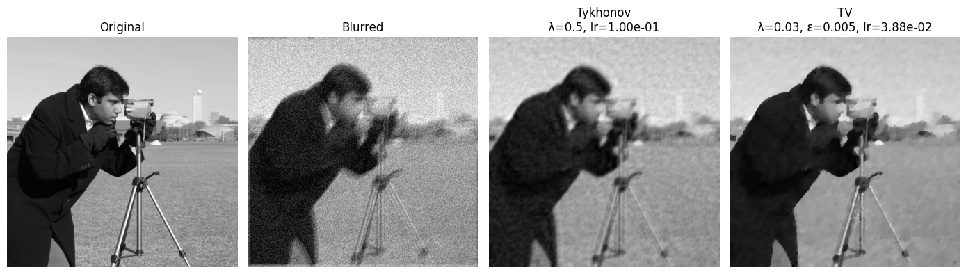
Denoising and deblurring formulated as optimization problems, solved in closed form in the Fourier domain and by gradient descent in PyTorch, comparing a quadratic smoothness prior with Total Variation.
Problem
A degraded image is modelled as v = A u + w, with u the clean image, A a degradation operator and w Gaussian noise.
The restored image minimizes a data-fidelity term plus a regularization:
û = argmin_u ½ ‖A u − v‖² + λ R(u)- Tikhonov,
R(u) = ‖∇u‖², is a quadratic smoothness prior with a closed-form solution in the Fourier domain. - Total Variation,
R(u) = Σ √(|∇u|² + ε²), favours sparse gradients and keeps sharp edges, but has no closed form.
Method
- Denoising (noise σ = 0.5): Tikhonov is solved both in closed form and by gradient descent. The two solutions are almost identical (17.87 dB against 17.95 dB at λ = 2, the gap coming from different boundary handling), which validates the gradient-descent code before applying it to Total Variation.
- Deblurring (known blur kernel, σ = 0.1): the convolution is computed by FFT, and both regularizers are solved by projected gradient descent.
- Step sizes come from the Lipschitz constant of each gradient, so no learning rate is tuned by hand.
- λ is chosen by sweeping a range of values and comparing images and metrics.
Results
| Task | Method | PSNR (dB) | SSIM |
|---|---|---|---|
| Denoising | Tikhonov, λ = 2 | 17.95 | 0.337 |
| Denoising | Total Variation, λ = 0.7 | 18.02 | 0.558 |
| Deblurring | Tikhonov, λ = 0.5 | 23.52 | 0.576 |
| Deblurring | Total Variation, λ = 0.03 | 25.07 | 0.668 |
Total Variation restores edges that Tikhonov smooths out, which shows mostly in SSIM. It costs more iterations and a second parameter, and it leaves flat, piecewise-constant patches in textured regions.