Relational learning on H&M sales

Two charts. Validation R² falls as message-passing hops are added, below LightGBM and close to persistence; removing the sales history drops R² from 0.563 to 0.048.

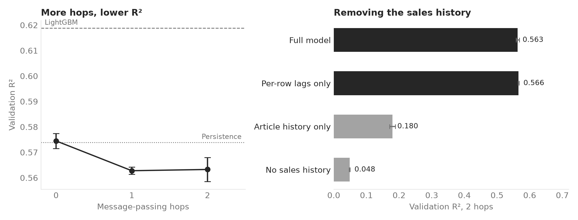
Do graph neural networks on a relational database beat a flat table with LightGBM? On H&M weekly article sales, a controlled ablation shows that the signal is autoregressive, not relational, and that the best graph model uses no message passing at all.

Key result: 0 hops is the best graph model, and LightGBM beats every graph configuration
Context: Télécom Paris team project on the RelBench benchmark (my part, the rel-hm dataset)
Team: ZHENG Tong, NARANJO RODRIGUEZ Natalia, SOUSSOU Koffi Désiré, CIZERON Jules and me, supervised by Nikola Simidjievski

Question

Relational deep learning treats a database as a graph and learns on it directly, instead of flattening the tables by hand. Our team tested whether this beats flat models on several RelBench tasks. I worked on rel-hm: H&M’s articles (105,542), customers (1.37 million) and transactions (15.2 million), with the task of predicting each article’s sales over the next 7 days. About 81% of the targets are zero.

Models

Persistence: next week’s sales are this week’s.
LightGBM on a flat table of article attributes, calendar features and sales lags.
HeteroSAGE, a heterogeneous GraphSAGE on the customer-article purchase graph, with a skip connection that feeds the article’s own sales lags straight to the prediction head. The full graph does not fit on a 16 GB GPU, so each article keeps 30 of its buyers, drawn at random with a new draw for each seed (1.31 million edges).

Results

Validation week, graph models averaged over 3 seeds:

Model	MAE	RMSE	R²
Persistence	0.0472	0.4323	0.574
LightGBM	0.0501	0.4089	0.619
HeteroSAGE, 0 hops	0.0572	0.4320	0.575
HeteroSAGE, 2 hops	0.0592	0.4377	0.563

Controlled ablation

With the architecture fixed, I varied only what the model can see, with 3 seeds per configuration:

The signal is autoregressive. Removing the sales history drops R² from 0.563 to 0.049.
The purchase graph carries a real but tiny signal. Without the sales history, going from 0 to 2 hops raises R² by 0.007, about 75 times less than the history.
With the history, the graph hurts. Going from 0 to 2 hops costs 0.011 of R², because averaging over an article’s buyers dilutes its own last-week sales.
It is not an artefact of the setup. A denser graph, other aggregators, down-weighting the second hop and richer node features all leave the 0-hop model ahead.

When the target is dominated by each entity’s own history, message passing is a noisy detour, and running a 0-hop control first is a cheap way to see it. On other tasks of the project, such as Formula 1 race results, the same method found that one hop carries most of the gain.

Limitations

One relation, one task and one validation week; aggregators limited to mean, sum and max; full-batch training that caps the graph density.

View the code Read the team report View the slides